\[ \newcommand{\set}[1]{\{\, #1 \,\}} \newcommand{\card}[1]{|#1|} \newcommand{\pset}[1]{𝒫(#1)} \newcommand{\falling}[2]{(#1)_{#2}} \]
Problem: Jump Up, Superstar!
In the reading, we explored Dijkstra’s algorithm, a fundamental technique for finding the shortest paths of a graph. Here, we explore the algorithm in more detail and then extend it to make it more appropriate for certain real world scenarios.
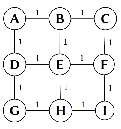
Run Dijkstra’s algorithm on the graph above, starting at vertex \(A\). In your write-up, give the resulting shortest paths and their costs from \(A\) to every other node in the graph.
In many cases, weights in our graph correspond to physical distances between vertices. In these scenarios, the triangle inequality will hold between vertices. For any three vertices \(a\), \(b\), and \(c\) that have edges between them, i.e., they form a triangle:
\[ |ab| + |bc| ≥ |ac| \]
where \(\card{ab}\) is the weight of edge \(ab\).
In a sentence or two, translate what the triangle inequality says with respect to the domain of vertices and lengths of paths between them.
In a sentence or two, explain why the graph from our previous lab on spanning trees:
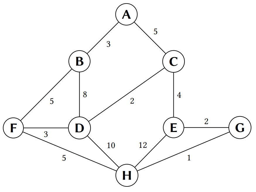
Does not obey the triangle inequality.
In cases where the triangle inequality holds, we can take advantage of this fact by introducing a heuristic function that allows us to better prioritize the nodes we consider during Dijkstra’s search. Let \(h(v)\) be the straight line distance between \(v\) and target \(t\). For example, in the graph from part (a), if we declare our target vertex to be \(I\), then:
\[\begin{align} h(A) &=\; h(A) = \sqrt{2^2 + 2^2} = \sqrt{8} \\ h(E) &=\; \sqrt{1^2 + 1^2} = \sqrt{2} \\ h(H) &=\; 1. \end{align}\]
all due to the Pythagorean theorem.
Rerun Dijkstra’s on this graph to find the optimal path from \(A\) to \(I\). However, when you need to calculate the next node to process, rather than choosing the minimal \(c(v)\), the current best-known path from \(A\) to \(v\), choose the vertex \(v\) that minimizes:
\[ c(v) + h(v). \]
In other words, choose the vertex \(v\) that minimizes the sum of the current best-known path from \(A\) to \(v\) and the straight line distance from \(v\) to \(I\). You may stop once you have established the shortest path from \(A\) to \(I\).
In your write-up, give the sequence of nodes that you visited in your modified algorithm. Also, in your write-up describe in a few sentences how the heuristic function \(h(v)\) made your shortest path search more efficient.
This extension of Dijkstra’s algorithm is called \(A^*\) (“A-star”) which is a common pathfinding algorithm in many contexts where the graph in question represents physical distances. In this problem, we considered a heuristic function \(h(v)\), but it turns out that any heuristic function will work as long as it doesn’t overestimate the actual cost to get to the goal node in the graph.
Discuss why the heuristic function must now overestimate the actual cost of the shortest path. Specifically, what happens to Dijkstra’s algorithm if the heuristic function has this bad property?